時間係列是每個數據點與時間戳相關聯的數據點。一個簡單的例子是股票在股票市場在不同的時間點在某一天的價格。另一例子是降雨量的區域中在不同月份的量。R輸入語言使用許多函數來創建，操縱和繪製時間序列數據。時間序列數據被存儲在R對象稱為時間序列對象。它也是類似向量或數據幀的R數據對象。

時間序列對象是通過使用 ts() 函數來創建。

語法

ts()函數時間序列分析使用的基本語法是：

timeseries.object.name <-  ts(data, start, end, frequency)

以下是所使用的參數的說明：

• data 包含在時間係列中使用的值的向量或者矩陣。
• start 指定開始時間在時間係列中。
• end 指定的結束時間的最後觀察的時間序列。
• frequency 指定的每個單位時間的觀測數。

除了參數“data”其他所有參數都是可選的。

示例

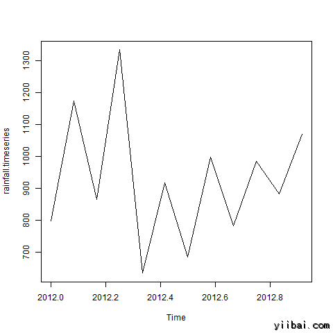
考慮從2012年1月開始，地方年降雨量細節。我們創造的R時間序列對象，期限為12個月，並繪製它。

# Get the data points in form of a R vector.
rainfall <- c(799,1174.8,865.1,1334.6,635.4,918.5,685.5,998.6,784.2,985,882.8,1071)

# Convert it to a time series object.
rainfall.timeseries <- ts(rainfall,start=c(2012,1),frequency=12)

# Print the timeseries data.
print(rainfall.timeseries)

# Give the chart file a name.
png(file = "rainfall.png")

# Plot a graph of the time series.
plot(rainfall.timeseries)

# Save the file.
dev.off()

當我們上麵的代碼執行，它會產生以下結果及圖表：

Jan    Feb    Mar    Apr    May    Jun    Jul    Aug    Sep
2012  799.0 1174.8  865.1 1334.6  635.4  918.5  685.5  998.6  784.2
        Oct    Nov    Dec
2012  985.0  882.8 1071.0

時間序列圖

不同的時間間隔

在頻率 ts() 函數參數的值 deices 的時間間隔，其中數據點被測量。 12表示的時間係列是12個月。 其他值和它的含義如下：

• frequency = 12 釘住數據點，一年中的每個月。
• frequency = 4 盯住數據點，每年每個季度。
• frequency = 6 釘住的數據點，一小時中每10分鐘。
• frequency = 24*6 釘住的數據點，每天中的每10分鐘。

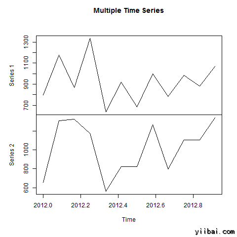
多時間序列

我們可以通過組合兩個串聯成一個矩陣的一個繪製多個時間序列圖表。

# Get the data points in form of a R vector.
rainfall1 <- c(799,1174.8,865.1,1334.6,635.4,918.5,685.5,998.6,784.2,985,882.8,1071)
rainfall2 <- c(655,1306.9,1323.4,1172.2,562.2,824,822.4,1265.5,799.6,1105.6,1106.7,1337.8)

# Convert them to a matrix.
combined.rainfall <-  matrix(c(rainfall1,rainfall2),nrow=12)

# Convert it to a time series object.
rainfall.timeseries <- ts(combined.rainfall,start=c(2012,1),frequency=12)

# Print the timeseries data.
print(rainfall.timeseries)

# Give the chart file a name.
png(file = "rainfall_combined.png")

# Plot a graph of the time series.
plot(rainfall.timeseries, main = "Multiple Time Series")

# Save the file.
dev.off()

當我們上麵的代碼執行，它會產生以下結果及圖表：

         Series 1 Series 2
Jan 2012    799.0    655.0
Feb 2012   1174.8   1306.9
Mar 2012    865.1   1323.4
Apr 2012   1334.6   1172.2
May 2012    635.4    562.2
Jun 2012    918.5    824.0
Jul 2012    685.5    822.4
Aug 2012    998.6   1265.5
Sep 2012    784.2    799.6
Oct 2012    985.0   1105.6
Nov 2012    882.8   1106.7
Dec 2012   1071.0   1337.8

多個時間序列圖